systemd is one of the most popular choices of service managers that acts as the init (PID=1) process on Linux distributions. Although some distributions prefer simpler alternatives such as OpenRC for Alpine Linux and Gentoo or BusyBox for embedded environments, chances are that you are using systemd at this moment.

One essential tool that systemd provides for profiling and debugging the boot process is systemd-analyze. Although this is more of a “Swiss army knife” kind of tool in that it can provide security recommendations for service isolation, s-can an display PCR registers of TPS, etc. we are going to use it strictly for figuring out the bottlenecks that prevent our system from booting faster.

Try to run the time sub-command of systemd-analyze. This will tell you how long it took for your system to reach userspace and start up all (relevant) services. Here, we have multiple stages enumerated:

1. firmware: This represents the time the BIOS / UEFI took to detect and initialize the hardware, run its Power On Self Test (POST) and load the next bootloader in the chain.
2. loader: This is most likely the time spent in GRUB. Note that not all bootloaders report this elapsed time. They need to implement systemd's Boot Loader Interface.
3. kernel: Fairly straightforward. It's the amount of time needed by the kernel to reach the point where it forks into userspace after being loaded into memory by the bootloader. During this time, hardware detection takes place, drivers are being assigned and initialized, and worker threads are being spawned.
4. userspace: This covers the critical service startup phase. May optionally include the rootfs pivot if an initial ramdisk is used.

What are your boot times and how would you go about optimizing each category?

Since the most likely candidate for optimization is usually the userspace component, let's take a look at the critical-chain sub-command. This feature will show us the most costly chain of dependencies that delay a certain unit. If no unit is passed as an argument, it will automatically select the default unit (i.e., graphical.target most likely).

Note however that each unit can have multiple dependencies but whose initialization is usually parallelized. Meaning that once you solve the most egregious delays, the critical chain may change to another path of the dependency tree.

graphical.target @10.072s
└─multi-user.target @10.072s
  └─docker.service @9.239s +832ms
    └─network-online.target @9.236s
      └─NetworkManager-wait-online.service @3.231s +6.003s
        └─ ...

In the example above we see that the default target is delayed primarily by the docker service that is waiting for the NetworkManager to be brought online. So a first step would be do disable it if it's not necessary immediately after boot. If you want to see the complete dependency tree from which a critical chain is selected, run the following command:

$ systemctl list-dependencies graphical.target

Identify your own critical unit chain and describe each elements that introduces a delay. Usually, these have a +<time> appended after their name and completion time. Can these units be disabled or are they critical to the initialization of the system?

Normally, static instrumentation has a steep learning curve and requires some prior knowledge of how compilers work. In this exercise we'll take a simpler approach. Instead of performing fine-grained instrumentation on a program's Abstract Syntax Tree (AST), we'll use a built-in gcc mechanism to only instrument functions on entry and exit.

By specifying the -finstrument-functions flag when compiling a certain source file, gcc will try to register hooks for every externally visible (i.e., not static) function in that Compilation Unit (CU). As a result, the following callbacks will be invoked before entering, or exiting each function, respectively. Definitions taken straight from the online documentation.

void __cyg_profile_func_enter (void *this_fn,
                               void *call_site);
void __cyg_profile_func_exit  (void *this_fn,
                               void *call_site);

If these functions are not defined or made available through a shared object, the program execution will not be impacted at all. If they are defined within the same CU where the instrumented functions are implemented, note that you should attach the no_instrument_function attribute to avoid infinite loops. If your program is written in C++ instead of C, make sure that you declare them as extern “C”. Otherwise, the symbol mangling of C++ will create ambiguities between the default declarations that the compiler will inject into the AST when encountering the instrumentation flag.

If you wish to learn more about static instrumentation we recommend this blog post that is one of the few good resources available for gcc. Although llvm is more popular for developing instrumentation / optimization passes, their API is a clusterfuck that changes every few months. gcc is more stable and does not require you to recompile the whole compiler in order to use them transparently. In contrast, the current pass manager in llvm can only load passes implemented as shared object plugins via opt (i.e., the llvm optimizer) which only works on llvm bitcode.

In the code skeleton for this lab, you will find an example application that performs an HTTP GET request and displays the response. With this application, we've also included an example implementation of instrumentation callbacks. Try to compile both of these and run the instrumented TCP client.

$ make
$ export LD_LIBRARY_PATH=$(realpath bin)
$ ./bin/http-get 23.192.228.80 80

First of all, notice that we've exported LD_LIBRARY_PATH. The reason for this is that the instrumentation callbacks reside in a shared object that is linked to the main executable. At runtime, ld-linux (i.e., the dynamic loader) will need a search path for it.

Also, note that we've hardcoded example.com as the Host header in the HTTP GET query, so make sure to provide a valid IP address. If you want to, you can patch the application source to make it more generic :p

After running the application, you should see something along these lines:

[*] src/ins/tool.cpp:35 Enter: (null) --> main
[*] src/ins/tool.cpp:35 Enter: main --> tcp_connect(char*, unsigned short)
[*] src/ins/tool.cpp:44 Exit : tcp_connect(char*, unsigned short) --> main
[*] src/ins/tool.cpp:35 Enter: main --> send_query(int, char const*, unsigned long)
[*] src/ins/tool.cpp:44 Exit : send_query(int, char const*, unsigned long) --> main

In our instrumentation callbacks, we use dladdr() to determine the symbol name of the function containing the call site / call target. This only works because we've specified the -rdynamic flag in the Makefile. This in turn passes -export-dynamic to the linker, telling it to add all symbols to the dynamic symbol table. Normally this helps when trying to obtain a backtrace from within a program. In our case, it allows to identify the functions involved in a call-based transition. Additionally, notice how some functions also contain the argument list. The reason for this is that we've also demangled the C++ symbols on your behalf.

Take a moment to analyze the source code and Makefile, then move on to the next task.

Time to get your hands dirty! Modify the instrumentation callbacks in a way that will allow you to measure the time spent in each function. In other words, measure the elapsed time between entering and exiting a function.

If one of these functions contains calls to other instrumented functions deduct their elapsed time. For example, after calculating the time that elapsed from entering until exiting main(), subtract the elapsed times of tcp_connect(), send_query() and recv_response(). For functions such as printf() that were not instrumented at compile time, there's noting to be done.

Add a destructor to the instrumentation callback library in which you will display these statistics when the program terminates.

Tracy is a feature-rich profiler that functions based on a client-server paradigm. The Server component is standalone and is used to analyze in real-time data collected during the execution of a program. When first started, the server will listen of a user-specified interface (default: loopback iface) for incoming connections from clients. The Client component must be embedded into your application. In other words, you must consciously designate the regions that need to be analyzed and the metrics that you want observed. The client code will continuously collect runtime information and send it to the server.

In this exercise we will walk through the process of adding Tracy support in an existing application, namely the OpenGL demo from the I/O monitoring lab. Specifically, we will observe the impact that doubling the number of vertices has on the CPU and GPU.

Because time is short and we can't explore each feature of Tracy, check out this interactive demo offered by the authors as a web-based Server with a pre-loaded trace.

Clone the Tracy project and jump into its root directory. Then, run the following commands to compile the Server component:

$ cmake -B profiler/build -S profiler -DCMAKE_BUILD_TYPE=Release 
$ cmake --build profiler/build --config Release --parallel

So far so good. Once we're done with the integration of the Client into our demo application, the Server will collect the trace data and process it for us. But first things first…

Go to lab_07/task_03/ where you will find a copy of the OpenGL application from our previous I/O monitoring lab. This version no longer has the tracking code that generated runtime statistics for you to plot.

The first step toward integrating Tracy with our OpenGL demo is to copy tracy/public/TracyClient.cpp in the project's src/ directory. Then, we're going to need access to some headers, so add -I${TRACY_DIR}/public to the CXXFLAGS variable in your Makefile.

Now that the compiler can find the headers, include tracy/Tracy.hpp in every source file that you want profiled (i.e., every other file in src/). Additionally, we must define the TRACY_ENABLE macro for the entire project in order for the profiler code to be compiled. Add -DTRACY_ENABLE to the CXXFLAGS in our Makefile.

Recompile the project and make sure you don't have any errors.

Now that we have the Tracy client code compiled into our application, it's time to add some markers. Because we defined the TRACY_ENABLE macro at a global scale, the FrameMark macro has the following definition in Tracy.hpp:

#define FrameMark tracy::Profiler::SendFrameMark( nullptr )

Place this macro at the end of the main rendering loop in the main() function of our demo app.

Similarly, place the ZoneScoped macro at the start of each function that you want included in the trace. This will include everything that executes within the scope of that function to the server, once FrameMark is reached.

Now that we've set up both the Server and the Client, it's time to test out Tracy. First, start tracy-profiler in your build directory from Task A. Hit the Connect button to listen for incoming connections from Clients on your localhost.

Next, start the demo application and hit ] a few times before exiting it. We want to generate a few events to identify on the Server.

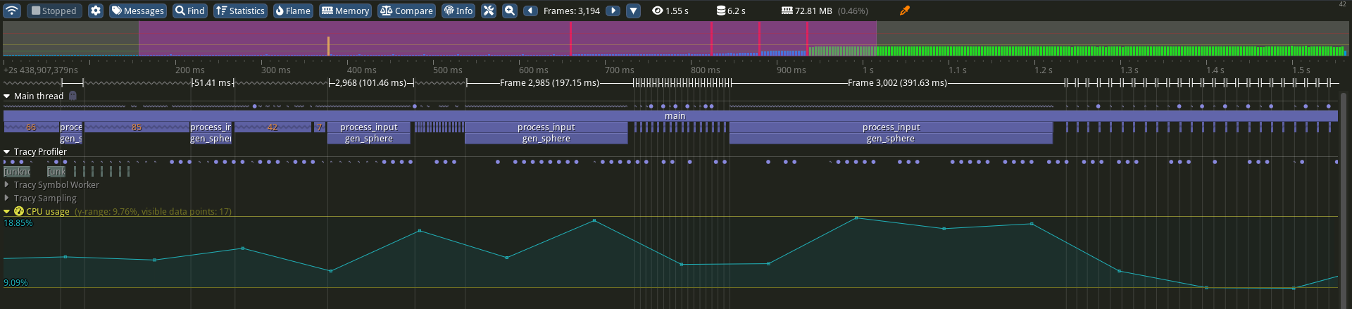
Because the Client that we integrated is bare-bones (i.e., cannot capture frames from the GLFW window, get GPU usage statistics, interpret DWARF symbols, etc.) the information seen in Figure 1 is limited in scope. However, we can point out how the duration of gen_sphere() becomes increasingly longer as we continuously double the amount of generated vertices. These function calls coincide with intervals of increased CPU activity. Also, notice how Tracy is able to unwind the call stack and determine that gen_sphere() is called as a result of processing input events in process_input(), inside the main rendering loop.

Now that we have our CPU profiling set up, it's time to add GPU support as well. Following this task, we will be able to identify the time slices in which the GPU is performing computations to satisfy our OpenGL draw requests. In order to figure this out, we need to add three additional Tracy macros in our main() function. These macros are defined in tracy/TracyOpenGL.hpp, so include it.

The three macros that you need to place inside the source code are as follows:

1. TracyGpuContext: Must be placed after GLFW window context & GLAD initializations. In other words, after glfwMakeContextCurrent() and gladLoadGLLoader(). Note that a limitation of Tracy is that it assumes that each thread has only one rendering context. In other words, a single-threaded application does not render two or more windows at the same time. In all fairness, this is usually the case.
2. TracyGpuZone(“NAME ME PLZ”): As most Tracy zone macros, it marks the current scope for a specific purpose. In this case, our macro will mark all functions from within its scope as API calls that queue work on the GPU. If you have doubts about what should be included inside this zone, check the code snipped below.
3. TracyGpuCollect: This macro will collect GPU the timings for the API calls located within any GPU zone. It should always be placed after swapping frame buffers. These timings will be communicated to the server and will be presented accordingly. Note that the return from glDrawArrays() let's say, does not coincide with the finalization of the GPU-bound work. That is why we need to obtain these exact timings.

/* draw points with the data stored in VAO */
glUseProgram(prog);
{
    TracyGpuZone("GPU draw");
    glUniform1f(theta_loc, 0.5f * glfwGetTime());
    glDrawArrays(GL_POINTS, 0, n);
}
 
/* swap front and back buffers & poll I/O events */
glfwSwapBuffers(window);
TracyGpuCollect;

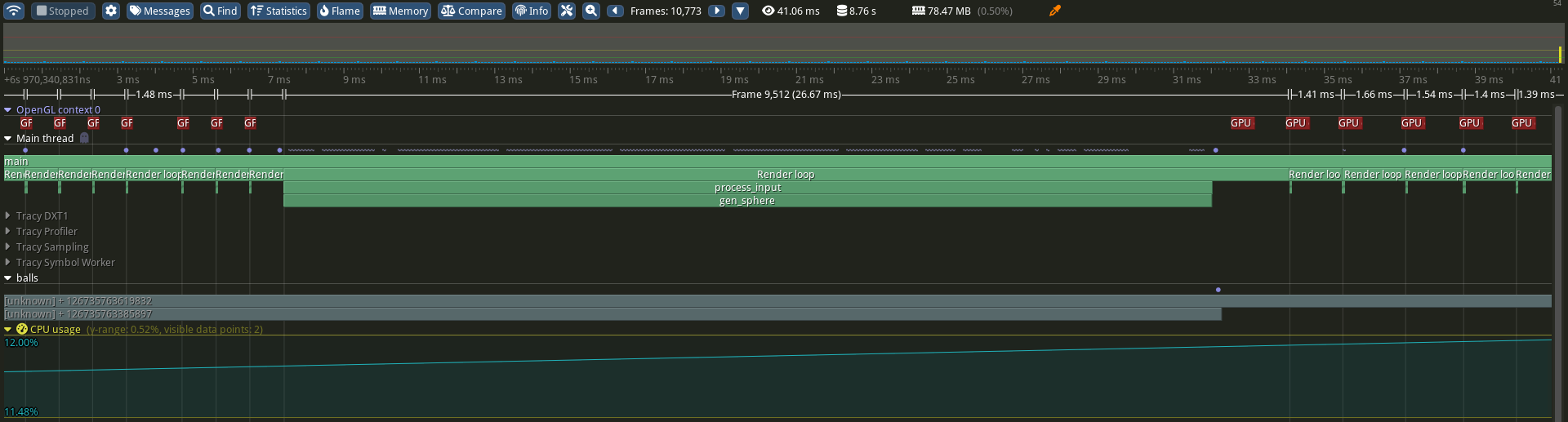
Extra task for you before you run your application again: Turn the scope of the main rendering loop into a named zone using the ZoneScopedN(“name”) macro. This should make it easier to visualize it on the Tracy server. You should obtain something along the lines of what you see in Figure 2. Notice how the duration of GPU-bound operations increased for every single draw command after regenerating the vertex coordinates. Keep in mind that we did not account for data transfers from RAM to vRAM that are triggered by glBufferData() in sphere.cpp.

The purpose of this exercise is to identify where bottlenecks appear in a real-world application. For this we will use perf and American Fuzzy Lop (AFL).

First, let's compile AFL and all related tools. We initialize / update a few environment variables to make them more accessible. Remember that these are set only for the current shell.

$ git clone https://github.com/google/AFL
 
$ pushd AFL
$ make -j $(nproc)
 
$ export PATH="${PATH}:$(pwd)"
$ export AFL_PATH="$(pwd)"
$ popd

Now, check that it worked:

$ afl-fuzz --help
$ afl-gcc --version

The program under test will be fuzzgoat, a vulnerable program made for the express purpose of illustrating fuzzer behaviour. To prepare the program for fuzzing, the source code has to be compiled with afl-gcc. afl-gcc is a wrapper over gcc that statically instruments the compiled program. This analysis code that is introduced is leveraged by afl-fuzz to track what branches are taken during execution. In turn, this information is used to guide the input mutation procedure.

$ git clone https://github.com/fuzzstati0n/fuzzgoat.git
 
$ pushd fuzzgoat
$ CC=afl-gcc make
$ popd

If everything went well, we finally have our instrumented binary. Time to run afl. For this, we will use the sample seed file provided by fuzzgoat. Here is how we call afl-fuzz:

• the -i flag specifies the directory containing the initial seed
• the -o flag specifies the active workspace for the afl instance
• -- separates the afl flags from the binary invocation command
• everything following the -- separator is how the target binary would normally be invoked in bash; the only difference is that the input file name will be replaced by @@

$ afl-fuzz -i fuzzgoat/in -o afl_output -- ./fuzzgoat/fuzzgoat @@

If you look in the afl_output/ directory, you will see a few files and directories; here is what they are:

• .cur_input : current input that is tested; replaces @@ in the program invocation.
• fuzzer_stats : statistics generated by afl, updated every few seconds by overwriting the old ones.
• fuzz_bitmap : a 64KB array of counters used by the program instrumentation to report newly found paths. For every branch instruction, a hash is computed based on its address and the destination address. This hash is used as an offset into the 64KB map.
• plot_data : time series that can be used with programs such as gnuplot to create visual representations of the fuzzer's performance over time.
• queue/ : backups of all the input files that increased code coverage at that time. Note that some of the newer files may provide the same coverage as old ones, and then some. The reason why the old ones are not removed when this happens is that rechecking / caching coverage would be a pain and would bog down the fuzzing process. Depending on the binary under tests, we can expect a few thousand executions per second.
• hangs/ : inputs that caused the process to execute past a timeout limit (20ms by default).
• crashes/ : files that generate crashes. If you want to search for bugs and not just test for coverage increase, you should compile your binary with a sanitizer (e.g.: asan). Under normal circumstances, an out-of-bounds access can go undetected unless the accessed address is unmapped, thus creating a #PF (page fault). Different sanitizers give assurances that these bugs actually get caught, but also reduce the execution speed of the tested programs, meaning slower code coverage increase.

Next, we will analyze the performance of afl. Using perf, we are able to specify one or more events (see man perf-list(1)) that the kernel knows to record only when our program under test (in this case afl) is running. When the internal event counter reaches a certain value (see the -c and -F flags in man perf-record(1)), a sample is taken. This sample can contain different kinds of information; for example, the -g option requires the inclusion of a backtrace of the program with every sample.

Let's record some stats using unhalted CPU cycles as an event trigger, every 1k events in userspace, and including frame pointers in samples:

$ perf record -e cycles -c 1000 -g --all-user \
    afl-fuzz -i fuzzgoat/in -o afl_output -- ./fuzzgoat/fuzzgoat @@

$ sudo su
$ echo -1 > /proc/sys/kernel/perf_event_paranoid
$ exit

Leave the process running for a minute or so; then kill it with <Ctrl + C>. perf will take a few moments longer to save all collected samples in a file named perf.data, which are read by perf script. Don't mess with it!

Let's see some raw trace output first. Then look at the perf record. The record aggregates the raw trace information and identifies stress areas.

$ perf script -i perf.data
$ perf report -i perf.data

Use perf script to identify the PID of afl-fuzz (hint: -F). Then, filter out any samples unrelated to afl-fuzz (i.e.: its child process, fuzzgoat) from the report. Then, identify the most heavily used functions in afl-fuzz. Can you figure out what they do from the source code?

Make sure to include plenty of screenshots and explanations for this task :p

A Flame Graph is a graphical representation of the stack traces captured by the perf profiler during the execution of a program. It provides a visual depiction of the call stack, showing which functions were active and how much time was spent in each one of them. By analyzing the flame graph generated by perf, we can identify performance bottlenecks and pinpoint areas of the code that may need optimization or further investigation.

When analyzing flame graphs, it's crucial to focus on the width of each stack frame, as it directly indicates the number of recorded events following the same sequence of function calls. In contrast, the height of the frames does not carry significant implications for the analysis and should not be the primary focus during interpretation.

Using the samples previously obtained in perf.data, generate a corresponding Flame Graph in SVG format and analyze it.

Please take a minute to fill in the feedback form for this lab.