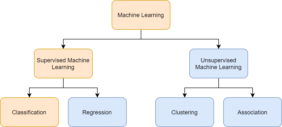
The purpose of an information system is to extract useful information from raw data. Data science is a field of study that aims to understand and analyze data by means of statistics, big data, machine learning and to provide support for decision makers and autonomous systems. While this sounds complicated, the tools are based on mathematical models and specialized software components that are already available (e.g. Python packages). In the following labs we will learn about.. learning. Machine Learning, to be more specific, and the two main classes: Supervised Learning and Unsupervised Learning. The general idea is to write software programs that can learn from the available data, identify patterns and make decisions with minimal human interventions, based on Machine Learning algorithms.

Supervised learning is the Machine Learning task of learning a function (f) that maps an input (X) to an output (y) based on example input-output pairs. The goal is to find (approximate) the mapping function so that new data can be predicted. The function can be continuous in the case of regression, or discrete in the case of classification, requiring different algorithms. Now, we will discuss about classification methods, where the input/output variables are attributes and not limited to numbers.

The main difference between them is that the output variable in regression is numerical (or continuous, such as “dollars” or “weight”) while that for classification is categorical (or discrete, such as “red”, “blue”, “small”, “large”). For example, when provided with a dataset about houses (e.g. Boston), and you are asked to predict their prices, that is a regression task because price will be a continuous output (see Lab 7). Examples of the common regression algorithms include linear regression, Support Vector Regression (SVR), and regression trees.

For example, when provided with a dataset about houses, a classification algorithm can try to predict whether the prices for the houses “sell more or less than the recommended retail price”. Examples of the common classification algorithms include logistic regression, Naïve Bayes, decision trees, and K Nearest Neighbors.

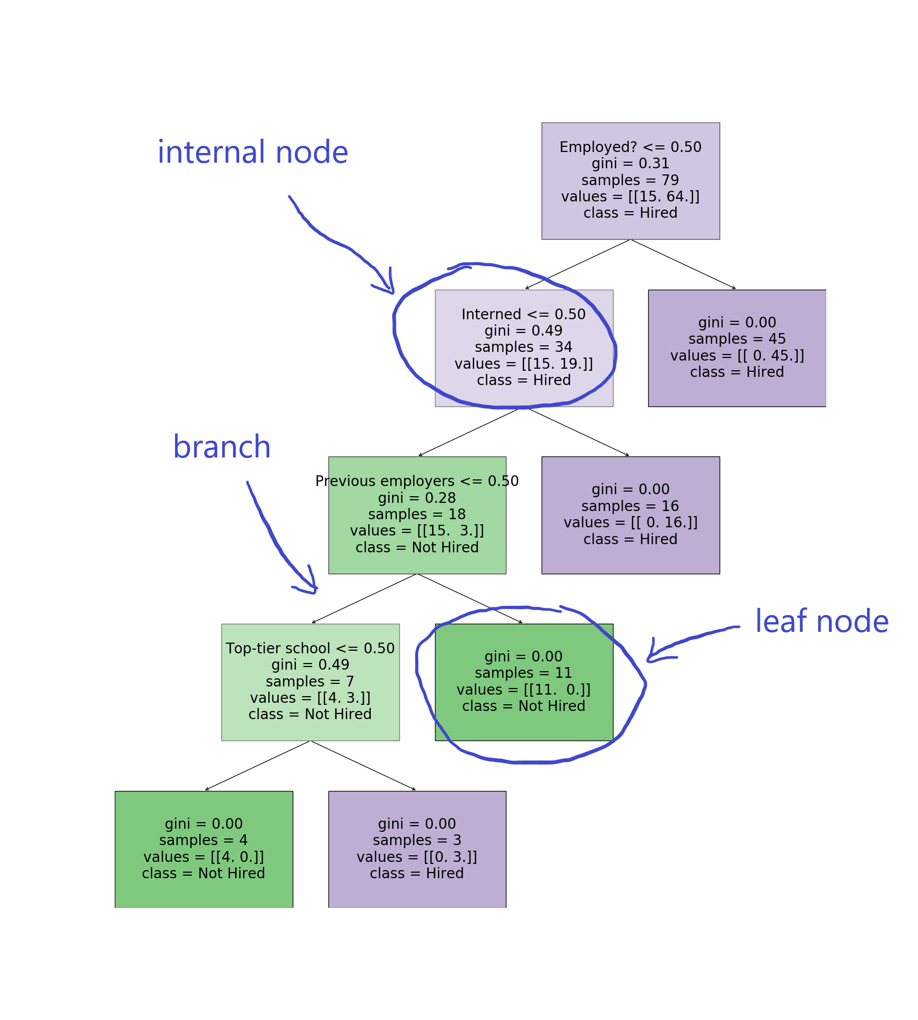
A decision tree is a classification and prediction tool having a tree like structure, where each internal node denotes a test on an attribute, each branch represents an outcome of the test, and each leaf node (terminal node) holds a class label:

• Input: historical data with known outcomes
• Output: rules and flowcharts (generated by the algorithm)
• How it works: the algorithm looks at all the different attributes and finds out the decisions that have to be made at each step in order to reach the target value.

Here is an example literally comparing apples and oranges based on the size and the texture of the fruit, based on Decision Trees. The algorithm has to learn from the available, labelled examples and then predict other fruits and classify them as either apples or oranges:

from sklearn import tree
 
# Gathering training data
c = {
    "rough": 0,
    "smooth": 1
}
 
o = {
    "apple": 0,
    "orange": 1
}
 
# scikit-learn requires real-valued features
features = [[155, c["rough"]], [180, c["rough"]], [135, c["smooth"]], [110, c["smooth"]]]
labels = [o["orange"], o["orange"], o["apple"], o["apple"]]
 
# training classifier
classifier = tree.DecisionTreeClassifier() # using decision tree classifier
classifier.fit(features, labels) # Find patterns in data
 
# making predictions
p = classifier.predict([[120, c["smooth"]]])
 
# showing results
inv_map = {v: k for k, v in o.items()}
p = [inv_map[e] for e in p]
print(p)

See the next example on how you can plot the decision tree:

# continue from previous example
 
# plot decision tree
from matplotlib import pyplot as plt
 
tree.plot_tree(classifier)
plt.show()

• A “forest” of decision trees
• Decision trees are susceptible to overfitting.
• One solution is to construct several trees and let them “vote” on the final classification.
• We do this by randomly re-sampling the input data for each tree (fancy term: bootstrap aggregating).

In Python (scikit-learn), we can just use the RandomForestClassifier instead of the DecisionTreeClassifier. There are some parameters that have to be defined such as the number of trees (n_estimators) and the random state (controls the randomness of the samples when building trees, set to 0 to disable)

from sklearn.ensemble import RandomForestClassifier
model = RandomForestClassifier(n_estimators=10, random_state=0)

You want to build a system to filter out resumes based on historical hiring data. You have a database of some important attributes of job candidates: Years Experience, Employed, Previous employers, Level of Education, Top-tier school, Interned, Hired. You can train a decision tree on this data, and arrive at a system for predicting whether a candidate will get hired based on it!

For this, the following steps are usually required:

• The dataset contained in a database/CSV file/other data source
• Data format and preprocessing
• Defining training, validation and test datasets
• Creating and training the Decision Tree
• Making predictions on the test dataset/new data

A decision tree is a classification and prediction tool having a tree like structure, where each internal node denotes a test on an attribute, each branch represents an outcome of the test, and each leaf node (terminal node) holds a class label.

The mapping function between input/output data can be represented as a flowchart. In this case study, a decision tree is trained on the HR dataset with the following visual representation:

Interpreting the data is straight-forward. At each “decision” (internal node) there are two branches: left (false), right (true) which represent the possible outcomes for the current test attribute (e.g. Interned). The leaf nodes are reached when all the samples are aligned to either outcome and hold the class labels (e.g. Hired/Not Hired) and shown with a different color for each class (in this case there are 2 classes: Hired/Not Hired). From the example, the decision for hiring a new candidate can be described as follows:

• If already employed
• If not already employed, but has interned at the company
• If not already employed, has not interned at the company, but has had previous employers
• If not already employed, has not interned at the company, has not had previous employers, but has been to a top-tier school

The data set may come in different formats, and it's recommended to have a common representation e.g. yes/no, true/false, can all be mapped to 1/0 binary representation, classes can be mapped to numbers, null values should be ignored (removed from the training data).

Here is an example that performs some data preprocessing on the HR dataset, mapping the employed status, and other indicators (input), as well as the hired result (output) to binary values: 1/0

import pandas as pd
 
input_file = "./data/past_hires.csv"
df = pd.read_csv(input_file, header=0)
 
# format the data, map classes to numbers
d = {'Y': 1, 'N': 0}
df['Hired'] = df['Hired'].map(d)
df['Employed?'] = df['Employed?'].map(d)
df['Top-tier school'] = df['Top-tier school'].map(d)
df['Interned'] = df['Interned'].map(d)
d = {'BS': 0, 'MS': 1, 'PhD': 2}
df['Level of Education'] = df['Level of Education'].map(d)
 
target = df['Hired']
 
print(target)

In Python we use the DecisionTreeClassifier from the scikit-learn package, that creates the tree for us. We train the model using the data set and then we can visualize the decisions. Then we can validate the model by comparing the target values to the predicted values, showing the prediction accuracy.

Here we continue the example with the HR dataset, and we are training a Decision Tree model to predict future hires:

from sklearn import tree
import numpy as np
 
# load the data (see previous example)
 
# print features and data
features = list(df.columns)
print("features: ")
print(features)
print("data: ")
print(df)
 
# prepare the data
X = df[features]
y = target
 
# now actually build the decision tree using the training data set
clf = tree.DecisionTreeClassifier()
clf.fit(X, y)

Download the Project Archive and install the required packages via requirements.txt

Run task1.py:

• The script loads the HR dataset described in the example, using the load_dataset function from loader.py, performs some preprocessing using the format_data function (mapping text data to numeric values for classification) and creates a decision tree classifier to predict future outcomes (Hired/Not Hired) using the create_decision_tree function from classifiers.py.
• The predictions are evaluated to find out the accuracy of the model and the decision tree is then shown as (pseudo)code (if else statements) and graph representation as dtree1.png.

Change the amount of data used for training the model and evaluate the results:

• prediction accuracy and generated output
• how large is the decision tree regarding the number of leaf nodes?

Run task2.py:

• The script loads the HR dataset described in the example (same as Task 1)
• The script creates and trains decision trees using variable amounts of training data (specified by the range: n_train_percent_vect). The accuracy for each case is saved into a list.
• The results are plotted on a chart, showing the effect of the amount (percent) of training data on the prediction accuracy

Evaluate the results:

• How much training data (percent) is required in this case to obtain the most accurate predictions?

Run task3.py:

• task3.py is similar to task1.py, using another dataset about wine quality: winequality_white.csv, winequality_red.csv to train a decision tree that should predict the quality of the wine based on measured properties.
• A brief description of the dataset:

Input variables (based on measurements):
1 - fixed acidity
2 - volatile acidity
3 - citric acid
4 - residual sugar
5 - chlorides
6 - free sulfur dioxide
7 - total sulfur dioxide
8 - density
9 - pH
10 - sulphates
11 - alcohol

Output variable (based on sensory data): 
12 - quality (score between 0 and 10)

Use n_train_percent to change the amount of data used for training the model and evaluate the results:

• prediction accuracy and generated output
• how large is the decision tree regarding the number of leaf nodes?

Create task4.py:

• task4.py is similar to task4.py and should evaluate the accuracy on the wine quality dataset using both decision trees and random forest models. The accuracy of the two models is compared on the plot for different amounts of training data, specified by n_train_percent.
• Run task4.py for both red (winequality_red.csv) and white (winequality_white.csv) wine datasets

Evaluate the results:

• How much training data (percent) is required in this case to obtain the most accurate predictions?
• What is the average accuracy for each model (decision tree, random forest)

Project Archive

https://data-flair.training/blogs/machine-learning-datasets/

https://archive.ics.uci.edu/ml/datasets/wine+quality